This page documents the syntax for Dynare 4.0. For later versions of Dynare, you need to use the new syntax for commands conditional_forecast, conditional_forecast_paths and plot_conditional_forecast, as documented in the reference manual.

Years ago I wrote three matlab files that allow to condition the DSGE forecasts on given future paths for a subset of endogenous variables. For instance:

• We may want to obtain a forecast with a fixed nominal interest rate.
• We may want to obtain a forecast with a given path of the relative price of oil.
• In a two country model, we may want to forecast domestic variables for a given path of the foreign variables or of the exchange rate.

This is done, from the reduced form representation of the DSGE model, by finding the structural shocks that are needed to match the restricted paths. An obvious limitations is that, working directly from the solution of a structural model, the households (or any other agents) do not use this information when they make their expectations and decisions. For instance, when we produce a forecast with a fixed nominal interest rate assumption, the agents believe instead that this variable will smoothly return to its steady state level. Put differently, the shock (the monetary policy shock in our example) used to satisfy the constancy of the nominal interest rate is a surprise for the agents.

Here is a(somewhat stupid)n example with a two country model where we constrain the paths of the nominal interest rates in the US and the Euro Area and the path of the nominal exchange rate. After the estimation command the user has to declare (i) the constrained endogenous variables, (ii) the shocks used to control the paths of these endogenous variables, (iii) the paths of the constrained endogenous variables, (iv) the number of periods during which a subset of endogenous variables is constrained, (v) the number of periods for the forecast, (vi) the number of simulations and (vii) the size of the confidence bands.

   //% DECLARATION OF THE CONSTRAINED ENDOGENOUS VARIABLES.
   cV = 'Robs';
   cV = strvcat(cV,'R_Fobs');
   cV = strvcat(cV,'NEER');
   //% DECLARATION OF THE EXOGENOUS VARIABLES USED TO CONTROL THE PATHS OF THE VARIABLES IN cV.
   //% NOTE: The ordering of the variables should not matter.
   cS = 'E_R';
   cS = strvcat(cS,'E_R_F');
   cS = strvcat(cS,'E_NEER');
   //% DECLARATION OF THE PATHS FOR THE VARIABLES IN cV.
   mcValue = zeros(size(cV,1),1);
   mcValue(1,1) = oo_.SmoothedVariables.Robs(end);
   mcValue(2,1) = oo_.SmoothedVariables.R_Fobs(end);
   cL = 8;            //% LENGTH OF THE CONSTRAINED PATH.
   H  = 40;           //% NUMBER OF PERIODS FOR THE FORECAST.
   B  = 10000;        //% NUMBER OF SIMULATIONS.
   ci = .80;          //% SIZE OF THE CONFIDENCE BANDS AROUND THE FORECASTS.
   imcforecast('mode',cV,cS,cL,H,mcValue,B,ci)

essai.m

Remark 1. In the third block, the paths are not declared for the eight periods but only for the first period (the nominal exchange rate -- in deviation to its steady state level -- is constrained to be zero, the nominal interest rates keep constant, using end of sample values). By default the routine will assume that the paths are constant over cL periods. Another scenario, with time varying paths may be defined as follows:

   path_for_the_first_variable = [.8 .9 .1 -.2 -.1 .2 .1 -.2];
   path_for_the_second_variable = [.31 .23 .27 .22 .18 .19 .23 .21];
   path_for_the_third_variable = [.32 .33 .37 .32 .38 .39 .29 .28];
   mcValue = [path_for_the_first_variable ; ...
              path_for_the_second_variable ; ...
              path_for_the_third_variable ];

Remark 2. The first argument of imcforecast is 'mode', 'mean' or 'median'. We do not consider the uncertainty on the deep parameters, so the user has to choose a point estimate for structural parameters (the posterior mode, the posterior mean or the posterior median).

Remark 3. Variables in cV and cS must be declared as endogenous variables and exogenous variables in the mod file.

Remark 4. Only observed variables should be constrained, I never tried to define the path of a latent variable (?? there is no test for this) .

The three matlab functions are in Dynare version 4.

How to build the plots?

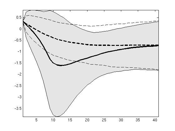
The function will save the results in a mat file called conditional_forecasts.mat. The user can obtain a plot for each endogenous variable by using the following instruction in the matlab command window:

plot_icforecast('Zobs')

where, in our example, Zobs is the US production. A plot like :

will pop up. The plain dark line is the mean of the conditional forecast and the shaded area represents the surface between the first and last deciles of the forecast distribution (if ci is set to eighty percent). The dashed dark line is the mean of the unconditional forecast. Note that the distribution of the constrained forecast is much more asymmetric than the distribution of the unconstrained forecast.

TODO list:

• Review imcforecast.m, icforecast3.m and plot_icforecast.m and add a description of the algorithm.
• Add the posterior uncertainty on the deep parameters (another loop is needed). Usually, the posterior uncertainty on the deep parameters affects only marginally the distribution of the (unconstrained) forecasts, so I do not expect big changes.
• Add an interface (modification of the preprocessor).

• It should be possible to build conditional forecasts from the structural representation of the model (so that, following our example, households know that the central bank will keep constant the nominal interest rate, say, for two years) using deterministic simulations. We just have to find anticipated paths for the subset of exogenous variables used to control the constrained endogenous variables (We need to find a fixed point -> another newton around the newton algorithm used to solve a deterministic model).

• It should be possible to estimate the DSGE model with constrained paths for a subset of the observed endogenous variables (out of sample information). We have to generalize the Kalman filter routines by allowing for missing observations (treated as latent variables).

Alternative approaches

• Junior Maih (2010) "Conditional Forecast in DSGE Models" paper