|
Size: 5872
Comment: Update link to Gitlab
|
← Revision 20 as of 2021-04-06 10:18:41 ⇥
Size: 5928
Comment: Fix typos in law of motion
|
| Deletions are marked like this. | Additions are marked like this. |
| Line 35: | Line 35: |
| \hat{Y}_t &=& L_t^\alpha (\hat{K}_{t-1}/(1+g_t))^\beta\\ | \hat{Y}_t &=& L_t^\alpha \left(\frac{\hat{K}_{t-1}}{1+g_t}\right)^\beta\\ |
| Line 40: | Line 40: |
| \hat{K}_t &=& (1-\delta)\hat{K}_{t-1}+\hat{I}_t | \hat{K}_t &=& \frac{(1-\delta)}{1+g_t}\hat{K}_{t-1}+{\hat{I}_t}^\frac{1}{\alpha+\beta} |
Stationarizing a non-linear model by hand is a tedious process that is better done by the computer.
Computing the equilibrium growth rates of a balanced growth model is complicated and will not be attempted here. We limit ourselves to replace non-stationary variables by their stationary counterpart as specified by the user.
Current restriction: for the time being we limit ourselves to stochastic trends integrated of order 1.
Simple example
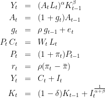
Original model
Consider a model with two trends: a labor productivity trend  and a nominal price trend
  .
.
The model is the following (some equations are omitted):

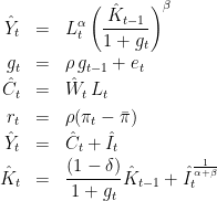
Stationarized model
We define stationarized variables by  ,
,  ,
,  ,
,  ,
,  .
.
The equations of the stationarized model are:

Note that the two trends  and
and  have disappeared from the model, along with their laws of motion.
Dynare syntax
Here is the syntax for writing the original (non-stationary) model in Dynare:
var g, pie;
trend_var(growth_factor=1+g) A;
trend_var(growth_factor=1+pie) P;
parameters alpha, beta, delta, rho, piebar;
var L, r;
var(deflator=A) K;
var(deflator=A^(alpha+beta)) Y C I;
var(deflator=P*A^(alpha+beta)) W;
varexo e;

model;
Y = (A*L)^alpha*K(-1)^beta;
g =rho*g(-1)+e;
P*C=W*L;
r =rho*(pie - piebar);
Y=C+I;
K=(1-delta)*K(-1)+I^(1/(alpha+beta));
//... and the last 3 equations
end;
Remarks:
- The trends are not declared as endogenous variables, but are attributed a new type.
- The order of declaration matters: the trend vars and some endogenous and parameters must be declared before the detrended variables.
Complete example
See fs2000_nonstationary.mod for a complete example using the cash-in-advance model of Schorfheide (2000).
Algorithm of transformation and test
- The algorithm is performed before introduction of auxiliary variables (because the preprocessor cannot guess the trends of auxiliary variables).
- Each detrended variable is replaced by itseft times its deflator (leading or lagging the deflator if the variable is itself leaded or lagged)
Then each leaded or lagged trend variable (declared with trend_var) is shifted to current period (by multiplying or dividing by the growth factor)
- A test is performed to check that the trends are compatible with balanced growth:
For all model equations
 , all trend variables
  and all dynamic endogenous variables
  , check that
  (by evaluating the derivative at the point given in initval; if you want the test to be effective, you should give values in initval such that the equations don't evaluate to NaN)
 - If any of the cross-derivatives is not null, the equation or the specification of trend for each variable is not compatible with balanced growth. Exit with an error message identifying the equation and the list of nonstationary variables affected by the faulty trend
If the test passed, replace trend variables (trend_var variables) by the value 1.
When the user wants to estimate the model in level, the user needs to introduce observed variables in level, but these should not be declared in trend_var nor be declared with a deflator.and not nonstationary variables must be linked to the stationarized variable via (log-)linear relations. For example, if Pobs is the observed price level, it should be a standard endogenous, with the equation:
Pobs/Pobs(-1)=1+pie;
And the trend of the observed variable must be declared with the trend keyword used for estimation:
observation_trends
P_obs (log(1+pie));
end;
For models written in logs
Sometimes you want to write your model in logs rather than in levels, and still use the automatic detrending engine. You can do this using the log_trend_var command and the log_deflator option of var.
Going back to the example at the top of this page, and supposing that all variables have been redefined as being equal to the log of the original variables (except for g, pie, r and e), the model can now be written as:
var g, pie;
log_trend_var(log_growth_factor=g) A
log_trend_var(log_growth_factor=pie) P;
parameters alpha, beta, delta, rho, piebar;
var L, r;
var(log_deflator=A) K;
var(log_deflator=(alpha+beta)*A) Y C I;
var(log_deflator=P+(alpha+beta)*A) W;
varexo e;

model;
Y = alpha*(A+L)+beta*K(-1);
g =rho*g(-1)+e;
P+C=W+L;
r =rho*(pie - piebar);
exp(Y)=exp(C)+exp(I);
exp(K)=(1-delta)*exp(K(-1))+exp(I)^(1/(alpha+beta));
//... and the last 3 equations
end;
(note that we have used the approximation  and
and  )
)