|
Size: 1159
Comment:
|
Size: 5736
Comment:
|
| Deletions are marked like this. | Additions are marked like this. |
| Line 1: | Line 1: |
| = Automatic removing of trends = |
|
| Line 7: | Line 5: |
| == First case: exogenous nonstationary process == | Current restriction: for the time being we limit ourselves to stochastic trends integrated of order 1. = Example = == Original model == Consider a model with two trends: a labor productivity trend <<latex($A_t$)>> and a nominal price trend <<latex($P_t$)>>. The model is the following (some equations are omitted): |
| Line 10: | Line 17: |
| y_t &=& A_t k_{t-1}^\alpha\\ | Y_t &=& (A_t L_t)^\alpha K_{t-1}^\beta \\ |
| Line 12: | Line 19: |
| g_t &=& \rho\, g_{t-1}+e_t | g_t &=& \rho\, g_{t-1}+e_t\\ P_t\,C_t &=& W_t\, L_t\\ P_t &=& (1+\pi_t) P_{t-1}\\ r_t &=& \rho (\pi_t - \bar{\pi}) \\ Y_t &=& C_t + I_t\\ K_t &=& (1-\delta)K_{t-1} + I_t^\frac{1}{\alpha+\beta} |
| Line 16: | Line 28: |
| Assuming that <<latex($y_t$)>> and <<latex($k_t$)>> have common trend <<latex($A_t$)>>, the stationarizing procedure calls for dividing first and second equation by <<latex($A_t$)>>. The second equation becomes meaningless and corresponds to the fact that <<latex($A_t$)>> doesn't belong to the stationary model. | == Stationarized model == |
| Line 18: | Line 30: |
| == Second case: endogenous nonstationary process {{{$!latex |
We define stationarized variables by <<latex($\hat{Y}_t = Y_t/A_t^{\alpha+\beta}$)>>, <<latex($\hat{C}_t = C_t/A_t^{\alpha+\beta}$)>>, <<latex($\hat{I}_t = I_t/A_t^{\alpha+\beta}$)>>, <<latex($\hat{K}_t = K_t/A_t$)>>, <<latex($\hat{W}_t = W_t/(P_t A_t^{\alpha+\beta})$)>>. The equations of the stationarized model are: {{{#!latex |
| Line 21: | Line 35: |
| P_t\,C_t &= W_t\, L_t\\ P_t &= (1+\pi_t) P_{t-1}\\ r_t &= \rho_1 (\pi_t - \bar \pi) |
\hat{Y}_t &=& L_t^\alpha (\hat{K}_{t-1}/(1+g_t))^\beta\\ g_t &=& \rho\, g_{t-1}+e_t \\ \hat{C}_t &=& \hat{W}_t\, L_t\\ r_t &=& \rho (\pi_t - \bar \pi) \\ \hat{Y}_t &=& \hat{C}_t + \hat{I}_t \\ \hat{K}_t &=& (1-\delta)\hat{K}_{t-1}+\hat{I}_t |
| Line 26: | Line 43: |
| In this case as well, the second equation becomes meaningless after stationarizing the model. | Note that the two trends <<latex($A_t$)>> and <<latex($P_t$)>> have disappeared from the model, along with their laws of motion. == Dynare syntax == Here are the proposed syntax for writing the original (non-stationary) model in Dynare: === Proposal 1 === {{{ var Y, L, K, g, C, W, pie, r, I; trend_var A, P; varexo e; parameters alpha, beta, delta, rho, piebar; trends; K: deflator=A, growth_factor=(1+g); Y, C, I: deflator=A^(alpha+beta), growth_factor=(1+g)^(alpha+beta); W: deflator=P*A^(alpha+beta), growth_factor=(1+pie)*(1+g)^(alpha+beta); end; model; Y = (A*L)^alpha*K(-1)^beta; g =rho*g(-1)+e; P*C=W*L; r =rho*(pie - piebar); Y=C+I; K=(1-delta)*K(-1)+I^(1/(alpha+beta)); //... and the last 3 equations end; }}} Remarks: * The trends are not declared as endogenous variables, but are attributed a new type. * In the {{{trends}}} block, the user has to specify both the expression used to detrend a given endogenous, then the growth factor of the same expression, followed by the corresponding variables. * The law of motion of trends in not in the {{{model}}} block (actually the same information is embedded in the {{{trends}}} block) === Proposal 2 === {{{ trend_var A, P; parameters alpha, beta, delta, rho, piebar; var L, g, pie, r; var(trend_deflator=A, trend_growth_factor=(1+g)) K; var(trend_deflator=A^(alpha+beta), trend_growth_factor=(1+g)^(alpha+beta)) Y C I; var(trend_deflator=P*A^(alpha+beta), trend_growth_factor=(1+pie)*(1+g)^(alpha+beta)) W; varexo e; model; Y = (A*L)^alpha*K(-1)^beta; g =rho*g(-1)+e; P*C=W*L; r =rho*(pie - piebar); Y=C+I; K=(1-delta)*K(-1)+I^(1/(alpha+beta)); //... and the last 3 equations end; }}} Note that the order of declaration matters: the trend vars and some endogenous and parameters must be declared before the detrended variables. = Algorithm of transformation and test = * The algorithm is performed after introduction of auxiliary variables to reduce leads and lags over multiple periods. * For each equation, in a temporary copy of the tree of this equation: 1. each variables appearing in the {{{trends}}} block is multiplied by the expression declared in first position of the {{{trends}}} block * If the variabe appears with a lead, in addition, it is multiplied by the growth factor of the trend pushed forward by one period * If the variable appears with a lag, in addition it is divided by the growth factor at the current period 2. Test: for all model equations <<latex($F(\ldots)=0$)>>, all trend variables <<latex($A_{i,t}$)>> and all dynamic endogenous variables <<latex($y_{j,t+k}$)>>, check that <<latex($\frac{\partial^2 \log F}{\partial A_{i,t}\partial y_{j,t+k}}=0$)>> (by evaluating the derivative at some point, typically the values given in {{{initval}}}). If any of the cross-derivatives is not null, the equation or the specification of trend for each variable is not compatible with balanced growth. Send an error message identifying the equation and the list of nonstationary variables affected by the faulty trend 3. write the equation on the model tree, replacing all {{{trend_var}}} variables by the value {{{1}}}. * Question: should we change the name of the variable when stationarized? It would be clearer, but more complicated as well. The user would have to use the modified name of the variable in all subsequent instructions and we would have to keep two lists of variable names. So I think that we should keep the same names. * When the user wants to estimate the model in level, the nonstationary variables must be linked to the stationarized variable via (log-)linear relations: {{{#!latex \[ Pobs_t/Pobs_{t-1} = (P_t/P_{t-1})exp(\pi)\\ \] }}} where {{{P}}} is the stationarized price level. In that case, variable {{{Pobs}}} shouldn't be listed in a {{{trend}}} expression, but only {{{P}}} and the original equation {{{ Pobs/Pobs(-1)=P/P(-1); }}} shall be transformed in {{{ Pobs/Pobs(-1)=P/P(-1)*exp(pie); }}} assuming that we have {{{ trend (exp(pie)), P; }}} |
Stationarizing a non-linear model by hand is a tedious process that is better done by the computer.
Computing the equilibrium growth rates of a balanced growth model is complicated and will not be attempted here. We limit ourselves to replace non-stationary variables by their stationary counterpart as specified by the user.
Current restriction: for the time being we limit ourselves to stochastic trends integrated of order 1.
Example
Original model
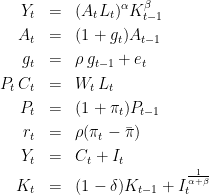
Consider a model with two trends: a labor productivity trend  and a nominal price trend
  .
.
The model is the following (some equations are omitted):

Stationarized model
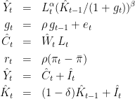
We define stationarized variables by  ,
,  ,
,  ,
,  ,
,  .
.
The equations of the stationarized model are:

Note that the two trends  and
and  have disappeared from the model, along with their laws of motion.
Dynare syntax
Here are the proposed syntax for writing the original (non-stationary) model in Dynare:
Proposal 1
var Y, L, K, g, C, W, pie, r, I;
trend_var A, P;
varexo e;
parameters alpha, beta, delta, rho, piebar;

trends;
K: deflator=A, growth_factor=(1+g);
Y, C, I: deflator=A^(alpha+beta), growth_factor=(1+g)^(alpha+beta);
W: deflator=P*A^(alpha+beta), growth_factor=(1+pie)*(1+g)^(alpha+beta);
end;

model;
Y = (A*L)^alpha*K(-1)^beta;
g =rho*g(-1)+e;
P*C=W*L;
r =rho*(pie - piebar);
Y=C+I;
K=(1-delta)*K(-1)+I^(1/(alpha+beta));
//... and the last 3 equations
end;
Remarks:
- The trends are not declared as endogenous variables, but are attributed a new type.
In the trends block, the user has to specify both the expression used to detrend a given endogenous, then the growth factor of the same expression, followed by the corresponding variables.
The law of motion of trends in not in the model block (actually the same information is embedded in the trends block)
Proposal 2
trend_var A, P;
parameters alpha, beta, delta, rho, piebar;
var L, g, pie, r;
var(trend_deflator=A, trend_growth_factor=(1+g)) K;
var(trend_deflator=A^(alpha+beta), trend_growth_factor=(1+g)^(alpha+beta)) Y C I;
var(trend_deflator=P*A^(alpha+beta), trend_growth_factor=(1+pie)*(1+g)^(alpha+beta)) W;
varexo e;

model;
Y = (A*L)^alpha*K(-1)^beta;
g =rho*g(-1)+e;
P*C=W*L;
r =rho*(pie - piebar);
Y=C+I;
K=(1-delta)*K(-1)+I^(1/(alpha+beta));
//... and the last 3 equations
end;
Note that the order of declaration matters: the trend vars and some endogenous and parameters must be declared before the detrended variables.
Algorithm of transformation and test
- The algorithm is performed after introduction of auxiliary variables to reduce leads and lags over multiple periods.
- For each equation, in a temporary copy of the tree of this equation:
each variables appearing in the trends block is multiplied by the expression declared in first position of the trends block
- If the variabe appears with a lead, in addition, it is multiplied by the growth factor of the trend pushed forward by one period
- If the variable appears with a lag, in addition it is divided by the growth factor at the current period
Test: for all model equations
 , all trend variables
  and all dynamic endogenous variables
  , check that
  (by evaluating the derivative at some point, typically the values given in initval). If any of the cross-derivatives is not null, the equation or the specification of trend for each variable is not compatible with balanced growth. Send an error message identifying the equation and the list of nonstationary variables affected by the faulty trend
 write the equation on the model tree, replacing all trend_var variables by the value 1.
- Question: should we change the name of the variable when stationarized? It would be clearer, but more complicated as well. The user would have to use the modified name of the variable in all subsequent instructions and we would have to keep two lists of variable names. So I think that we should keep the same names.
- When the user wants to estimate the model in level, the nonstationary variables must be linked to the stationarized variable via (log-)linear relations:
![\[
Pobs_t/Pobs_{t-1} = (P_t/P_{t-1})exp(\pi)\\
\] \[
Pobs_t/Pobs_{t-1} = (P_t/P_{t-1})exp(\pi)\\
\]](/DynareWiki/RemovingTrends?action=AttachFile&do=get&target=latex_35e7ed7ab2b1b4a25a9e5bd65293b75b47a50bd0_p1.png)
where P is the stationarized price level. In that case, variable Pobs shouldn't be listed in a trend expression, but only P and the original equation
Pobs/Pobs(-1)=P/P(-1);
shall be transformed in
Pobs/Pobs(-1)=P/P(-1)*exp(pie);
assuming that we have
trend (exp(pie)), P;