|
Size: 2376
Comment:
|
← Revision 10 as of 2009-03-25 17:12:09 ⇥
Size: 2380
Comment: converted to 1.6 markup
|
| Deletions are marked like this. | Additions are marked like this. |
| Line 30: | Line 30: |
| attachment:trace_plot.jpg | {{attachment:trace_plot.jpg}} |
| Line 32: | Line 32: |
| where the black curve is a moving average of the sampled values. That is, if the sampled values are [[latex($\{\alpha_i\}_{i=1}^N$)]] where [[latex($N$)]] is the number of simulations in the Metropolis Hastings chain, the moving average curve is defined as: | where the black curve is a moving average of the sampled values. That is, if the sampled values are <<latex($\{\alpha_i\}_{i=1}^N$)>> where <<latex($N$)>> is the number of simulations in the Metropolis Hastings chain, the moving average curve is defined as: |
| Line 38: | Line 38: |
| for all [[latex($j$)]] between [[latex($q+1$)]] and [[latex($N-q$)]]. The default value of [[latex($q$)]] is 200. The value of [[latex($q$)]] may be changed by writing: | for all <<latex($j$)>> between <<latex($q+1$)>> and <<latex($N-q$)>>. The default value of <<latex($q$)>> is 200. The value of <<latex($q$)>> may be changed by writing: |
| Line 42: | Line 42: |
| before the call to trace_plot. A value of [[latex($q$)]] roughly equal to [[latex($10 \%$)]] of [[latex($N$)]] seems to be reasonable. In our example, we see that the moving average curve is slightly downward slopping, meaning that the Metropolis Hastings did not reach the ergodic distribution after 22000 draws. | before the call to trace_plot. A value of <<latex($q$)>> roughly equal to <<latex($10 \%$)>> of <<latex($N$)>> seems to be reasonable. In our example, we see that the moving average curve is slightly downward slopping, meaning that the Metropolis Hastings did not reach the ergodic distribution after 22000 draws. |
How to obtain trace plots after a Metropolis-Hastings
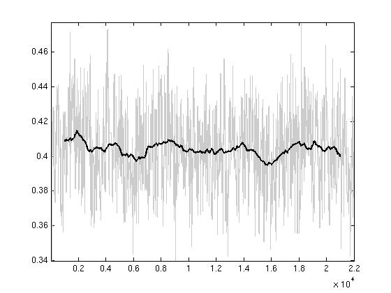
It can be useful to plot iterations vs. sampled values for each variable (parameter) in a chain. If the Metropolis-Hastings converges to a stable distribution, the trace plot has to be stable (e.g. no trend in the sampled values).
After a metropolis (that is after the estimation command in the mod file) you just have to write:
trace_plot(options_,M_,estim_params_,type,blck,name1,name2)
where:
- options_, M_ and estim_params_ are Dynare's global structures describing the model,
type is a string equal to 'DeepParameter' (for a parameter of the structural model), 'MeasurementError' (std. or correlation in the measurement equation error) or 'StructuralShock' (for the standard deviation of a structural shock or the correlation between two shocks),
blck<mh_nblck is an integer specifying the mh chain to be considered,
- name1 is a string specifying for instance the name of a deep parameter,
- name2 is an optional second string needed if you are interested in the correlation between two structural shocks or two measurement errors.
After the estimation of the model in fs2000.mod if we want to build a trace plot for parameter alp, we write:
trace_plot(options_,M_,estim_params_,'DeepParameter',2,'alp')
and the following plot will pop up:

where the black curve is a moving average of the sampled values. That is, if the sampled values are  where
where  is the number of simulations in the Metropolis Hastings chain, the moving average curve is defined as:
![\[
a_{j}=\frac{1}{2q+1}\sum_{k=-q}^{q} \alpha_{j+k}
\] \[
a_{j}=\frac{1}{2q+1}\sum_{k=-q}^{q} \alpha_{j+k}
\]](/DynareWiki/TracePlots?action=AttachFile&do=get&target=latex_098c69828fc9cafdc4f847f6f25402de3f45c6b6_p1.png)
for all  between
  and
and  . The default value of
  is 200. The value of
  may be changed by writing:
options_.trace_plot_ma = 2222;
before the call to trace_plot. A value of  roughly equal to
  of
of  seems to be reasonable. In our example, we see that the moving average curve is slightly downward slopping, meaning that the Metropolis Hastings did not reach the ergodic distribution after 22000 draws.